Daily Notes: 2025-11-27

ML Notes

In which we test whether the perceptron converged and visualize the decision boundaries for this 2-D dataset.

from matplotlib.colors import ListedColormap
from ml_utils.perceptron import Perceptron
import numpy as np
import pandas as pd
import matplotlib.pyplot as plt

s = 'https://archive.ics.uci.edu/ml/machine-learning-databases/iris/iris.data'
df = pd.read_csv(s, header=None, encoding='utf-8') # dataframe

# print(df.tail()) # just to ensure that the data was loaded correctly

# Goal here is to restrict the task to a binary classification problem
y = df.iloc[0:100, 4].values # creates a np array (.values) from the species labels (4 == 5th column == species) of the first 100 rows
y = np.where(y == 'Iris-setosa', 0, 1) # 0 if setosa, 1 if versicolor (first 100 rows only have those two species)

# Goal here is to extract two fairly separable features from the same 100 rows of y
X = df.iloc[0:100, [0, 2]].values # 100 x 2 matrix that extracts two features: sepal length (0) and petal length (2)

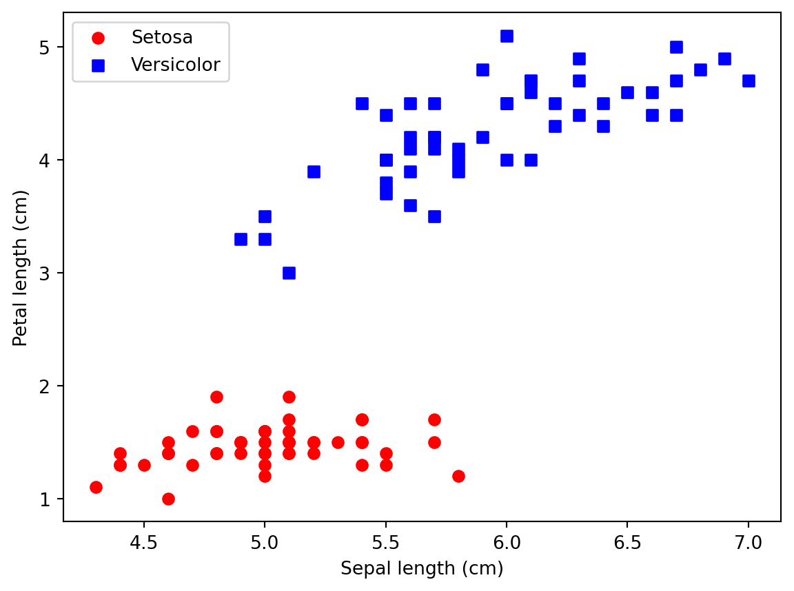
# Plot the two iris classes in the 100 x 2 matrix to visualize how separable they are before fitting a perceptron
# It's important that it's roughly linearly separable, which is when a perceptron would be a good choice

plt.scatter(X[:50, 0], X[:50, 1], color='red', marker='o', label = 'Setosa')
plt.scatter(X[50:100, 0], X[50:100, 1], color='blue', marker='s', label = 'Versicolor')

# Note that the x-axis here would be sepal length (because it's in column 0) and y-axis would be petal length (column 1)
plt.xlabel('Sepal length (cm)')
plt.ylabel('Petal length (cm)')
plt.legend(loc='upper left')
plt.show()

ppn = Perceptron(eta=0.1, n_iter=10)
ppn.fit(X,y) # train Perceptron on the Iris data subset

# Explore how the perceptron's training errors evolve over epochs.
# range(1, len(ppn.errors_) + 1) just creates the epoch numbers (x-axis)
plt.plot(range(1, len(ppn.errors_) + 1), ppn.errors_, marker='o') # draws a point for each training epoch
plt.xlabel('Epochs')
plt.ylabel('Number of updates')
plt.show() # Converges after 6th epoch

def plot_decision_regions(X, y, classifier, resolution=0.02):

    # setup marker generator and color map
    markers = ('o', 's', '^', 'v', '<')
    colors = ('red', 'blue', 'lightgreen', 'gray', 'cyan')
    cmap = ListedColormap(colors[:len(np.unique(y))])

    # plot the decision surface
    x1_min, x1_max = X[:, 0].min() - 1, X[:, 0].max() + 1
    x2_min, x2_max = X[:, 1].min() - 1, X[:, 1].max() + 1
    xx1, xx2 = np.meshgrid(np.arange(x1_min, x1_max, resolution),
                           np.arange(x2_min, x2_max, resolution))
    lab = classifier.predict(np.array([xx1.ravel(), xx2.ravel()]).T)
    lab = lab.reshape(xx1.shape)
    plt.contourf(xx1, xx2, lab, alpha=0.3, cmap=cmap)
    plt.xlim(xx1.min(), xx1.max())
    plt.ylim(xx2.min(), xx2.max())

    # plot class examples
    for idx, cl in enumerate(np.unique(y)):
        plt.scatter(x=X[y == cl, 0], 
                    y=X[y == cl, 1],
                    alpha=0.8, 
                    c=colors[idx],
                    marker=markers[idx], 
                    label=f'Class {cl}', 
                    edgecolor='black')


plot_decision_regions(X, y, classifier=ppn)
plt.xlabel('Sepal length [cm]')
plt.ylabel('Petal length [cm]')
plt.legend(loc='upper left')

plt.show()

NoteReusable code

This chunk pulls the Perceptron class from code/ml_utils/perceptron.py. Keeping reusable models in code/ lets Quarto posts stay lean while GitHub readers can browse the source directly.

Personal Notes

• There are two ways to run Python files:
  • python script.py runs the file directly.
  • python -m package.module runs it as part of a package (which makes package-style imports work).
• Think of your project as a bookshelf full of Python packages. When you run python script.py, you’re saying “open this file by its path.” Python doesn’t automatically know where that file sits on the shelf, so package-style imports may fail.
  • When you run python -m ml_utils.plot_decision_regions, you’re saying “look on the shelf for the ml_utils package, take the plot_decision_regions module out, and run it.” Because Python finds the module through the package, it automatically knows about ml_utils and any sibling modules. That’s why relative or absolute imports inside the module work—they’re being run “inside” the package instead of as a standalone file.
• A good setup: keep experimental scripts in an experiments/ folder and run them with python -m experiments.some_script from the project root. That way they can import things from ml_utils without extra tricks.

NotePython tips

• A module is just a single .py file. For example, perceptron.py or plot_decision_regions.py each define functions/classes and can be imported with their filename (minus .py).
• A package is a folder that contains modules (and usually an __init__.py file). It lets Python treat the folder as a single namespace so you can import things like ml_utils.perceptron.
• The package provides structure and a shared namespace; the modules are the individual files inside it. When you run python -m ml_utils.plot_decision_regions, you’re telling Python to execute the plot_decision_regions module as part of the ml_utils package, so it knows how to resolve imports like from ml_utils.perceptron import Perceptron.

Questions I still have

• Need to resist the urge to brush up on Python basics in a 101 bottom-up style.

Tomorrow’s plan

• I asked GPT-5.1 Codex to analyze my notes thus far and outline a path for what’s to come:
  • Finish the perceptron loop: add dataset splits (train/test or cross-validation), compute accuracy/confusion matrices, and document failure cases when classes aren’t separable. This turns the current script into a minimal experiment you can evaluate.
  • Feature scaling & preprocessing: implement standardization pipelines to see how learning rate, convergence, and decision boundaries change, especially before moving beyond Iris.
  • Logistic regression & soft margins: move from perceptron to logistic regression or linear SVMs to understand probabilistic outputs, loss functions, and regularization—natural evolutions of your current model.
  • Multi-class strategies: prototype OvA or OvO wrappers around your perceptron/logistic models to reinforce how binary learners extend to multi-class tasks.
  • Experiment tracking: start logging hyperparameters, metrics, and plots (even in your daily notes) so you build the habit of reproducible ML experiments.
  • Deepen EDA intuition: answer your own question by comparing outcomes with and without exploratory plots—note when simple visuals caught issues early versus when they weren’t needed.