Daily Notes: 2025-12-20
ML Notes
Bias Variance & Regularization
The five-step process that the authors propose in the paper Prediction of Advertiser Churn for Google AdWords:
- Select samples for analysis
- Define churn and select features (potential explanatory variables)
- Process data: transform features and impute missing values
- The goal of the third step is to generate more discriminating/relevant features to predict churn. This can be done via linear or non-linear transformations. Some examples are PCA, LDA, data preprocessing.
- Build predictive models
- Evaluate trained models
Bias Variance
- Underfitting: High Bias
- Overfitting: High Variance
- Think of bias in ML as a algorithm’s preconception of the shape of the model.
- Think of variance in ML as how much the model might change based on new data. For a regression model, if it’s overfit on your dataset, then new data will lead to a wildly different model.
- Workflow: Fit an algorithm that’s “quick & dirty” then understand whether it’s high bias or high variance and improve it.
- Regression models & Classification models are both subject to bias variance.
Regularization
The Linear Regression Objective Function (“Least Squares Cost Function”) is:
\(\min_{\theta}\; \frac{1}{2}\sum_{i=1}^{m}\left\|y^{(i)}-\theta^{T}x^{(i)}\right\|^{2}\)
- \(\min_{\theta}\): Choose a \(\theta\) that minimizes the total squared residual magnitude across all training examples.
- \(\frac{1}{2}\) doesn’t change the minimizer, and is included for algebraic convenience (to get rid of the factor of 2 when differentiating a squared term)
- \(\sum_{i=1}^{m}\) is the sum across \(m\) training examples
- With linear regression, the predictor \(\hat{y}^{(i)}\) is the dot product \(\theta^{T}x^{(i)}\). This is the guess of the model. It is linear with the parameters in that \(\theta\) only appears to the first power. This is very important! Optimization becomes harder (you can use gradient descent for local minima) with non-linear parameters.
- If \(y^{i} \in \mathbb{R}\) (a scalar output), then the Euclidean norm \(\left\| \right\|\) is redundant (you can use \((...)\) instead).
- But given that \(y^{i} \in \mathbb{R}^{k}\) (a vector output), then you need the Euclidean norm.
To add Regularization, you add a regularization term:
\(\min_{\theta}\; \frac{1}{2}\sum_{i=1}^{m}\left\|y^{(i)}-\theta^{T}x^{(i)}\right\|^{2} + \lambda\left\|\theta\right\|^{2}\)
Sometimes you write multiply \(\lambda\) by \(\frac{1}{2}\) to make derivation easier:
\(\min_{\theta}\; \frac{1}{2}\sum_{i=1}^{m}\left\|y^{(i)}-\theta^{T}x^{(i)}\right\|^{2} + \frac{\lambda}{2}\left\|\theta\right\|^{2}\)
- The advantage of adding a small \(\lambda\) (say, \(\lambda = 1\)) is that it penalizes \(\theta\) from being too big. Therefore, it makes it harder for the learning algorithm to overfit the data.
- If \(\lambda\) is too big (say, \(\lambda = 1000\)), however, you risk underfitting the data.
Personal Notes
Self-directed projects are hard to understand where to begin, so I read two papers for examples of Classification: Prediction of Advertiser Churn for Google AdWords and Building Airbnb Categories with ML and Human-in-the-Loop.
For the AdWords paper, I found it interesting that the definition of “customer churn” was not well-defined.
The challenge with top-down learning is that groping around in the dark can be incredibly demotivating. Watching the Stanford lectures felt like a breath of fresh air. I was also able to focus more effectively than just openly learning. Seems like the optimal balance is to have both.
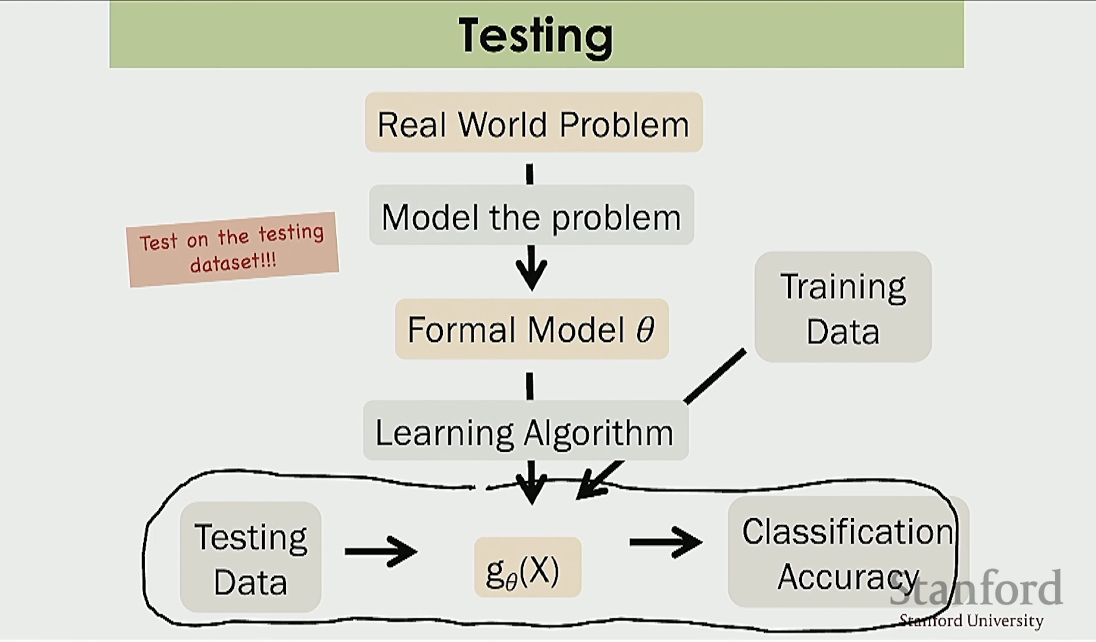
Used Andrew Ng’s lectures on data splits to understand how to split data for my project.
Used Chris Piech’s lecture to understand Logistic Regression.